Coupled atmosphere-ocean models
- This page is part of the topic Models of the physical and biological environment of the Antarctic
Predictions of future climate changes can only be made by using coupled global climate models (GCMs). These are also primary tools with which to simulate the past and present-day climates. Simulation of present day climates by these models provides a way of rigorously testing their ability to reproduce reality. Such reality checks are often crude, given that most of the commonly used GCMs do not operate at a finer scale than one-degree squares.
There are two main classes of coupled climate models: models of reduced complexity (see Claussen et al., 2002[1]) and three-dimensional coupled atmospheric and oceanic general circulation models. In the following text, coupled atmosphere-ocean models means three-dimensional coupled atmospheric and oceanic general circulation models. These models are continually evolving so as to more closely reflect reality, through improvements to resolution on the one hand, and to increases in the number of potentially interacting properties of the climate system used in each model on the other hand.
In the early 1990s, there were only a few coupled global climate models; by 2006, as noted in the fourth assessment report of the Intergovernmental Panel on Climate Change (IPCC, 2007[2]), around 24 such models were available to join the model inter-comparison project. Here we give a brief description of a coupled atmosphere-ocean model, and discuss their strengths and weaknesses, before presenting some results relevant to the Antarctic from the models used in the IPCC AR4.
A coupled atmosphere-ocean model or climate model has generally four major components: the atmosphere, the ocean, the land surface and the ice (cryosphere). More components are now being added to coupled models, such as biogeochemistry, in order to simulate the carbon cycle, and atmospheric chemistry.
The atmospheric component of such a model consists of a dynamical core that uses the equations of momentum and thermodynamics expressed in a set of partial differential equations, along with many physical processes, to observe change through time away from a set of initial conditions. The horizontal components of these partial differential equations are often solved using spectral methods on a supercomputer or network of PCs. Typically the horizontal resolution is 2o to 3o. In the vertical direction, variables are held on surfaces of constant pressure or height, or on surfaces that follow the orography. Typically, there are 20 to on order of 100 levels in the vertical direction. The water cycle and cloud-radiation interactions play very important roles in the climate system (e.g. clouds can both reflect incoming solar radiation, and absorb outgoing infrared radiation from the Earth’s surface), but they are two of the largest areas of uncertainty in the current generation of climate models. Processes operating at the sub-grid scale, such as the formation of cumulus clouds, have to be parameterized using the quantities that the model can resolve. Since the processes of cloud formation are not well understood, there are many uncertainties in these parameterizations – nevertheless their adequacy can be tested by their ability to simulate known modern conditions.
The oceanic component has many similarities to the atmospheric element, apart from the fact that the ocean is seen as a basin with side boundaries. To compensate for the existence of these side boundaries, the equations are solved using finite difference methods in the horizontal direction, with a typical resolution of 1-2o. In the vertical direction, most models use height as a coordinate, although some models use quasi-isopycnic coordinates (equal density) (for example, in the Miami Isopycnal Coordinate Ocean Model). Usually 20-40 levels are used in the current generation of models. Because sea water is much denser than air, ocean currents are much slower than winds, and a much higher spatial resolution is needed to resolve the processes happening in the ocean on the same time scale as the processes operating in the atmosphere. The details of the physical processes that need to be represented in the atmospheric and oceanic components determines the computing resources per grid square for each domain. It is still a matter of debate to what extent variations of small scale turbulence, sea ice properties, brine rejection etc have to be represented in large scale ocean models.The typical spatial scale of mesoscale eddies in the ocean is around 10 km, which is too fine to be resolved by the ocean components of GCMs. Eddy processes in the ocean, like clouds in the atmosphere, therefore have to be parameterised. However, the differences between results with models of different resolution suggests that the present parametrisations are far from being perfect. Eddy processes are important, because they are actively involved in the buoyancy and momentum transport across the ACC and in the boundary layers.
The land-surface component of GCMs is important in the global energy and water balance. Land surface temperature and soil moisture content are two basic variables in the energy and water exchanges between the atmosphere and the land surface. Some key properties including the roughness and albedo (reflectivity) are usually prescribed from the observed datasets. Some prescribed key properties can now be interactively determined in coupled models. For example, a dynamic global vegetation model can produce active vegetation types that can be used to determine the likely surface roughness and albedo. Land surface processes can also strongly affect the oceanic heat and freshwater fluxes.
Sea ice and snow over land are two important elements that are explicitly modeled in coupled GCMs. Glaciers and ice shelves are usually not resolved; instead, large-scale ice sheets (including ice shelves) are prescribed as land-surface topography with a high albedo. In addition to a high surface albedo, sea ice has very important insulation effects that inhibit the momentum, heat and freshwater exchanges between the ocean and the atmosphere. Sea ice formation or melting has strong effects on the freshwater flux. Early coupled climate models had very simple sea ice models, but recently more coupled GCMs employ sea ice models with more complex thermodynamics and sea ice dynamics.
Initialization
Initial conditions are needed for the ocean component because it is a slowly varying component. Observed present-day ocean temperature and salinity are usually used to initialize the ocean component. Another slowly varying component, the continental ice sheet is prescribed in terms of the present-day condition.
Flux adjustment
After the initial conditions are provided, the model is coupled together by allowing the exchanges of momentum, heat and freshwater between the atmosphere and ocean. In the early days of the development of coupled models, it was necessary to adjust the momentum, heat and freshwater fluxes to avoid large drifts of the model steady state away from the present-day climate. The use of flux adjustments was due to the existence of relatively large errors, mainly in the atmosphere and ocean components, and the fact that errors in one component could lead to further errors in the other components. Today, most coupled climate models have improved to the point where they no longer need to use flux adjustments.
Although significant progress has been made, large errors in the coupled models still exist, especially in southern high latitudes. For example, in the UK Hadley Centre climate model (HadCM3), the drifts of atmospheric and oceanic heat transport are largest in the southern high latitudes (see Figure 16 of Gordon et al., 2000[3]). It is difficult to represent small-scale topographic features over the Antarctic and in the Southern Ocean, yet these play key roles in steering currents and ice streams. Shelf processes are believed to be very important in the Antarctic deep/bottom water formation and need to be represented correctly in models. Melting and freezing at the base of ice shelves are completely unrepresented in the current generation of coupled climate models; the role played by sea ice in the southern high latitude water cycle is untreated, because of the lack of observed sea ice volume and sea ice drift velocity. As a result the various models have large uncertainties, and the simulated fluxes of freshwater into the ocean are highly varied. Currently no model can realistically resolve the Antarctic ice sheet and ice shelves and their effects on the ocean circulation.

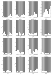
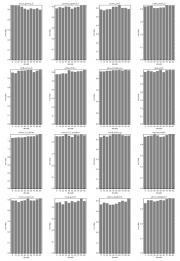
Ocean circulation simulation is still variable across the range of models. ACC transport is significantly biased in most IPCC AR4 models (Russell et al., 2006a[5]). The simulated strength of the largest sub-polar gyre - the Weddell Gyre, has a very different value in different models (Figure 2.31). The changes of the Weddell Gyre strength during the 20th century in 18 AR4 models are also shown in this figure. The mean precipitation over the Antarctic and its change in 18 AR4 models is shown in Figure 2.32. Sea ice extents simulated by AR4 models are also very different (see Parkinson et al., 2006[6]).
A correct simulation of the Antarctic climate needs correct representation of the atmosphere, ocean and cryosphere components. The interactions between these components are very complicated and difficult to represent in models. Over the last 50 years changes in surface temperature across the Antarctic have been dominated by the winter season warming on the western side of the Antarctic Peninsula. The ensemble mean of the IPCC AR4 models when run through this period with natural and anthropogenic forcing correctly identified this area as having some of the largest warming in the Antarctic. However, the magnitude of the warming was only about a quarter of that observed in reality and there were very large differences between the models. As we discuss below, part of the problem is that the resolution of the GCMs is very coarse, preventing us from resolving features such as the Antarctic Peninsula, where some key climate changes are known to be occurring.
In addition there is still a dearth of appropriate observations against which to test models. The IPY 2007-2008 provided an opportunity for climate modellers to further validate and improve their models, and provided additional insights to improve understanding of the complex climate system in the southern high latitudes. Before we are able to point out the future directions of the model improvements, we have to have enough observational data to assess the model performance. In the meantime, more model intercomparison work needs to be carried out to find out the model ensemble means and the model differences.
References
- ↑ Claussen, M. Et AL. 2002. Earth system models of intermediate complexity: closing the gap in the spectrum of climate system models, Clim. Dyn., 18, 579-586.
- ↑ 2.0 2.1 IPCC 2007. Climate Change 2007: The Physical Science Basis. Contribution of the Intergovernmental Panel on Climate Change. Cambridge University Press, Cambridge.
- ↑ Gordon, D.A., Priscu, J. and Giovannoni, S. 2000. Origin and phylogeny of microbes living in permanent Antarctic lake ice, Microb. Ecol. 39, 197-202.
- ↑ Klatt, O., Fahrbach, E., Hoppema, M. and Rohardt, G. 2005. The transport of the Weddell Gyre across the Prime Meridian, Deep-Sea Research II, 52, 513-528.
- ↑ Russell, J.L., Stouffer, R.J. and Dixon, K.W. 2006a. Intercomparison of the Southern Ocean circulation in IPCC coupled model controm simulations, J. Clim., 19, 4560-4575.
- ↑ Parkinson, C.L., Vinnikov, K.Y. and Cavalieri, D.J. 2006. Evaluation of the simulation of the annual cycle of Arctic and Antarctic sea ice coverages by 11 major global climate models, J. Geophys. Res., 111, doi:10.1029/2005JC003408.
